
Sampling survey to the total area of the forest of Heshun county in Shanxi province in year 2000
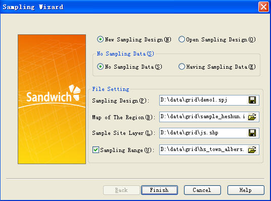
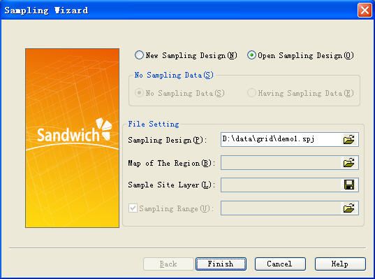
Defaults: “ New Sampling Design"> No Sampling Data ”, set the file as follows:
“ Sampling Design ” is the file that save the sampling design data, created and named by user, its postfix is.prj;
“Map of the region” is the RS image of the prepared sampling zone (it is .img format);
“Sample Site Layer” is the file that save the sample sites this time, created and named by user, its postfix is.shp
The selected sampling model is simple random sampling
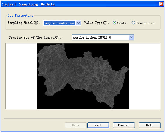
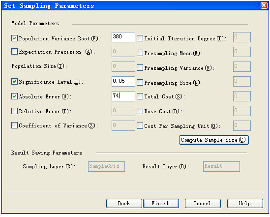
Figure 3.Set the sampling parameters
In this interface, all parameters can be set according to the requirements of user.
In this case, “Population Variance”、“Confidence Level (namely, Significance level of confidence)” and “Absolute Error” re needed to be set. (Population variance is the estimated value of the previous investigated results, which is known)
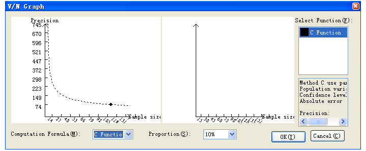
Then click the button of “Compute Sample Size”, enter the calculation interface of samples. In this interface, select “Function C” ( The program automatically invokes this function according to the parameters inputted by the user ) to calculate.
Step 4: Browse the sampling sites
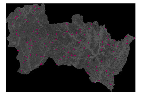
After clicking “Finish” in the back step, the software automatically pop the Feature table of the sampling sites and the spatial distribution graph, click the sampling design defined by user, which is in the “Data Source” of “Working Space Manager” in the left, this file involves the imported and created file in the sampling process , click the customed site layer file, then see the sampling site file, click the imported file of the Map of the region, then see the sampling sites of the whole area.
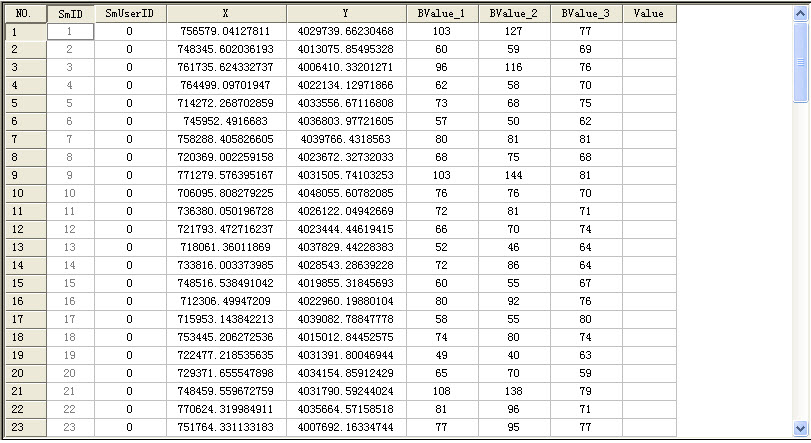
In Figure 5, the two columns in the table ( SmID 、 SmUserID) are automatically created by Supermap, the first column is the internal order of the data record, the second column is the order that signify the record by user, which can be modified according to the requirement, X 、 Y is latitude and longitude of the sampling sites, Bvalue1 Bvalue2 Bvalue3 are the different wave of the image, the value is the grey level of this sample site in these waves, “Value” is the investigated forest area of this sample site, which need to be inputted by user.
Hereto, distributing the sampling sites is finished. User can do field investigation according to the sampling sites, and gain the required sample data.
Step 5: Close the opened data source, open the sampling wizard dialog, click and open the existed sampling file, open the new sampling design in the place of sampling design, namely, the .spj file defined by user.
Step 6: Input the sampling site data. In Figure 8, Bvalue1 Bvalue2 Bvalue3 are the different waves of the image, the value is the grey level of this sample site in these waves, “Value” is the investigated forest area of the sample.
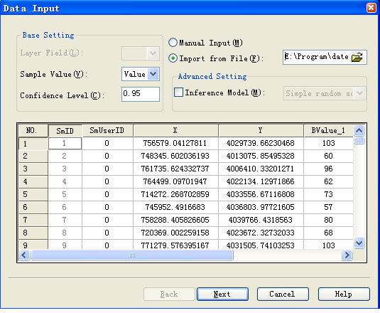
Select the sample values, there are two input ways, user can input by hand or import from the file, and input the confidence level.
User can select the other statistical inference models according to the requirement.

Calculation is completed. (Because the sampling sites are generated randomly each time, and the change of each sample site is larger, the screenshots results and the calculation results may be not complete agreement)
Note: Before creating the new project file or importing the existed one, user need to close the opened project file.