- Double-click
 SSSampling.
Pop-up under interface:
SSSampling.
Pop-up under interface:
- Under "Sample Design": click on
 ,
choose a suitable file path to save the project files, such as: “sampling project”
,
choose a suitable file path to save the project files, such as: “sampling project”
- Under "The Map of The Region": click on
 ,
choose the hs_town.shp file
,
choose the hs_town.shp file
- Under "Sample Site Layer": click ,
choose a suitable file path and input the saved file of the sample sites, such as: samping sites
2 - 4 steps, as shown below:
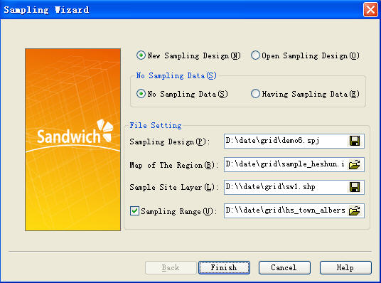
- Click on the "Finish"
- Note: If at this time a sample range file and the map of the region of interest is area based object, there will be no need to change the sampling range settings. If the map of the region is site based object, then the sampling range should includes the object region for sample site .(for example, the sampling site is samlingframe.shp, the sample range is hs_county.shp)
-
After the previous step have been completed, click out of the following interface

- Choose “ Sandwich sampling model”, pop-up under window:
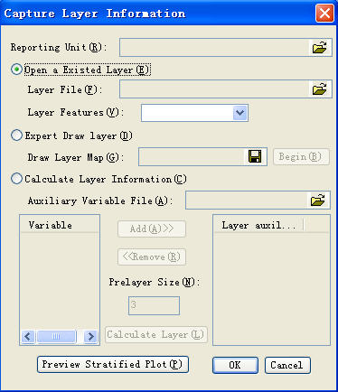
There are three ways to set up stratification, but only one may be used at a time.
i. Open stratification: open the selected the stratification, then click to open the stratification file, pop-up dialog box. The selected stratification file must be the object of the regional set. The stratified region must coincide with the map of region interest, then select stratification feature that is, identification of the different stratification features.
ii. Expert drawing stratification: first to create a new file to save the expert drawing stratification. Then click start drawing, the software will return to the map of region interest, experts draw the broken line to divide the map of region interest into a number of sub-regions. The each of sub-region is a stratum.
iii. Calculating stratification information: select stratification information, open assisted variable information file. According to certain features of the stratification of the file, the features in the table will be added to the right of the window, enter the number of layers before stratification( The default is 3), click the calculation of stratification to obtain the result of stratification.
Click on "preview stratification map", we can see the result of stratification.
- Set sampling resolution as 0.01, move pop-up window, you can see in the middle of map of the region of interest there is a small box, this is the smallest sampling unit based on input sample resolution. According to input different sample resolution, the size of the box will change in real time(if map of the region of interest is site based object, there's no need to set up sampling resolution)
-
Click "Scale" (or proportion of value determined by target
value)
- Click "Next"
-
After the previous step have been completed, pop-up following interface.
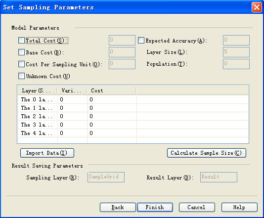
- Input parameters and verify the correctness of the input parameters. When click "Unknown Cost", cann't fill out the cost
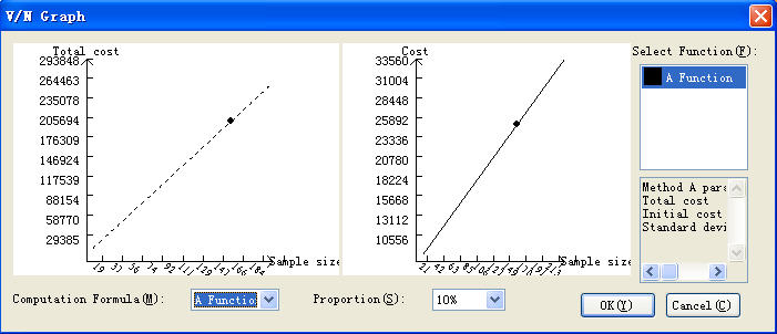
- Click on the "Compute Sample Size," and obtain the relationship graph between precision and sample size and cost. as shown below
- Select a different function, obtain a different sample precision relationship graph
-
Click on the name of calculation functions, we can see that each
function uses different parameters
- Select "Proportion", which is the actual number of samples compared to the theoretical value, as shown below
-
Click on “Back” to return the parameters interface, can modify
parameters
- Click on the "Finish", determined sample function
- Back to the design parameter interface, click "Finish", complete sample size calculation and system will generate sample site
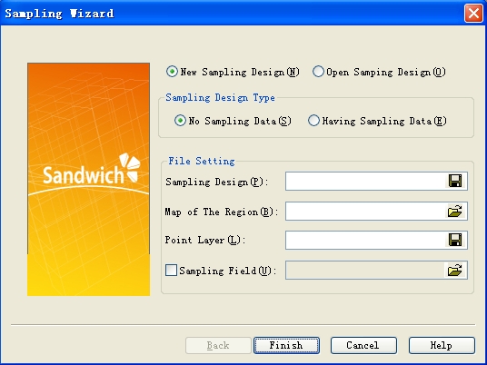
- Double-click SSSampling.
launch pop-up interface:
-
Select " Open Sampling Design ", open the project file which
generated in the first step.

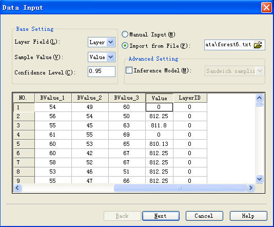
- Click OK, click out of the pop-up dialog for data input.
-
Select "Import from File
", open the saved data file (the file format is
txt), then select the property of the calculation value (generally
value)
- Or select manually input file, enter value directly under the value field in the form. Then select the property of calculation value.
- Sampling model has two kinds of situations
i. Directly click" Next", obtain sampling results
ii. Select sampling model, and then select spatial random model, get different results. Or choose spatial, spatial stratified and sandwich layered model, this time pop-up dialog box, which need to enter the relevant stratification file(for example: If the data is in order, natural stratification file using stritify.shp, reporting unit using hs_town.shp which only used in the sandwich model).
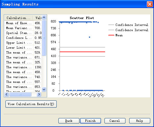
- Click “ Next”, show up a sampling results map: